Cellular Automata in MGS

Cellular Automata (CA for short) is a computing model used in a theoretic perspective in fundamental computer science as well as a modeling/simulating tool. A CA consists of a regular lattice of cells, each cell being characterized by its local state. The mapping of a state to each cell of the network (in other words, the global state of the CA) is called a configuration. The dynamics of the CA is specified through local rules allowing the evaluation of the next state of cell as function of its current state and the state of a finite number of neighbors. One of the most important point in CA is that cells behave synchronously: they all switch to their next state at the same time.

MGS topological collections and transformations can be seen as a weakening of CA (from regular grid to arbitrary neighborhood, from local rules to transformation rules, from synchronicity to a rewriting strategy). This make the language suitable for expressing CA as illustrated by the examples below.

To illustrate the adequacy of MGS to express CA, we propose to focus on the modeling of fire spread in forest. In the following two models are implemented:

• a simple but paradigmatic 3-state CA
• a more elaborated model due to Karafyllidis & Thanailakis

In this CA, a cell represents either some plants, or some fire or ashes. The rule are extremely simple:

• a forest cell gets in fire if one of its neighbors is burning
• a fire cell turns to ashes

Let define the filename for JBView visualization

ofile := "/tmp/ff.jbv" ;;

Cells have three possible states: forest, fire, ash

type cell = `Forest | `Fire | `Ash ;;
 
type configuration = [cell]Moore ;;

Let define a initialization function populating a given grid g with 0 and 1 at random

fun populate_grid(g:Moore, size_x:int, size_y:int) = (
 
  for i = 0 to size_x do
    for j = 0 to size_y do
      g.(i * |E> + j * |N>) := if random(10000) < 5 then `Fire else `Forest fi;
  g
 
) ;;

Let define the initial state S0

S0 := populate_grid(Moore:(),100,100) ;;
 
configuration(S0);;

The previous code uses the predefined GBF topological collection Moore which corresponds to an infinite square grid with 8 neighbors; to switch to a von Neuman neighborhood (infinite square grid with 4 neighbors, called NEWS in MGS) do

type configuration = [cell]NEWS ;;
 
fun populate_grid(g:NEWS, size_x:int, size_y:int) = (
 
  for i = 0 to size_x do
    for j = 0 to size_y do
      g.(i * |East> + j * |North>) := if random(10000) < 5 then `Fire else `Forest fi;
  g
 
) ;;
 
S0 := populate_grid(NEWS:(),100,100) ;;

Let define the cellular automaton rules

trans rules = {
 
  // Fire propagates to neighbor forest cells
  `Forest as c / neighbors_exists(equal(`Fire), c) => `Fire;
 
  // Extinction of fire
  `Fire => `Ash;
 
} ;;

Let define a function to save data for the viewer

fun output(S) = (
 
  ofile << " { " ;
  foreach c @ p in S do
    begin
      let (x,y) = sequify(p) in
        ofile << " { " << x << " " << y;
        ofile << switch c
                 case `Forest: " 0.6  0.73 0.35 } "
                 case `Fire:   " 0.96 0.59 0.27 } "
                 case `Ash:    " 0.29 0.27 0.16 } "
                 endswitch
    end;
  ofile << " }\n" ;
  S
 
) ;;

Let save data during the simulation

rules[fixpoint,
      prelude = output,
      interlude = output
     ](S0) ;;

The whole code follows

ff.mgs

ofile := "/tmp/ff.jbv" ;;
 
type cell = `Forest | `Fire | `Ash ;;
type configuration = [cell]Moore ;;
 
fun populate_grid(g:Moore, size_x:int, size_y:int) = (
 
  for i = 0 to size_x do
    for j = 0 to size_y do
      g.(i * |E> + j * |N>) := if random(10000) < 5 then `Fire else `Forest fi;
  g
 
) ;;
 
S0 := populate_grid(Moore:(),100,100) ;;
 
configuration(S0);;
 
trans rules = {
 
  // Fire propagates to neighbor forest cells
  `Forest as c / neighbors_exists(equal(`Fire), c) => `Fire;
 
  // Extinction of fire
  `Fire => `Ash;
 
} ;;
 
fun output(S) = (
 
  ofile << " { " ;
  foreach c @ p in S do
    begin
      let (x,y) = sequify(p) in
        ofile << " { " << x << " " << y;
        ofile << switch c
                 case `Forest: " 0.6  0.73 0.35 } "
                 case `Fire:   " 0.96 0.59 0.27 } "
                 case `Ash:    " 0.29 0.27 0.16 } "
                 endswitch
    end;
  ofile << " }\n" ;
  S
 
) ;;
 
rules[fixpoint,
      prelude = output,
      interlude = output
     ](S0) ;;

I. Karafyllidis and A. Thanailakis¹⁾ proposed an elegant but realistic model of fire spread which takes into account some environmental effects like wind (for both speed and direction), type of fuel, and landscape topography. The model is specified as a CA where the state of a cell is characterized by the ratio of burnt area ranging continuously from 0 (wholesome forest) to 1 (burnt forest - ashes) where the interval (0,1) represents burning forest.

karafyllidis_thanailakis_ff.mgs

////////////////////////////////////////////////////////////
// DEFINITION OF THE SYSTEM
 
N := 100 ;;
 
SCALE := 10000 ;;
 
rose := |N>,|NE>,|E>,|SE>,<N|,<NE|,<E|,<SE|,():ring ;;
 
trans searchPos[v] = {
  x / (x==v) => return(^x)
} ;;
 
// Wind
 
type wind = [float]Moore ;;
 
fun new_wind(dir:posgbf, force:(`Strong|`Weak|`None)) = (
 
  let (d,md,orth,diag,mdiag) =
    if (force == `Weak) then (0.9,1.1,1.0,1.0,1.04)
    elif (force == `Strong) then (0.5,1.8,1.0,0.7,1.3)
    else (1.0,1.0,1.0,1.0,1.0) fi
  in
  let p = searchPos[v=dir](rose) in
    {| d     @ rose.(p),
       md    @ rose.(p+4),
       orth  @ rose.(p+2),
       orth  @ rose.(p-2),
       diag  @ rose.(p+1),
       diag  @ rose.(p-1),
       mdiag @ rose.(p+3),
       mdiag @ rose.(p-3)
    |}:Moore
 
) ;;
 
// State
 
type       system = [cell]Moore
and record cell   = {
  wind:wind,
  burnt:float,
  height:float,
  rate:float
}
and record burnable = cell + { burnt ~= 1.0 } + { rate ~= 0.0 }
and record burnt    = cell + { burnt  = 1.0 }
;;
 
// Specification of a configuration constructor
fun new_grid(f) = (
  reverse(fold((\i,acc.(
    reverse(fold((\j,acc.(  f(i-1,j-1) :: acc  )),seq:(),N)) :: acc
  )),seq:(),N)) following |E>, |N>
) ;;
 
fun export_grid[ofile="/tmp/toto"](color,g) = (
  stdout << "iteration: " << 'iteration << "\n";
  ofile << " { " ;
  fold((\i,acc.(
    fold((\j,acc.(  let c = color(g.((i-1)*|E> + (j-1)*|N>)) in
      if c <> WHITE then
        ofile << " { " << (i-1) << " " << (j-1) << " " << c.r << " " << c.g << " " << c.b << " } "
      fi
    )),<undef>,N)
  )),<undef>,N) ;
  ofile << " } " ;
  g
) ;;
 
fun color(v) =
  if   burnt(v)       then WHITE
  elif v.burnt == 0.0 then WHITE
  else mult_color(WHITE,GRAY(1.0-v.burnt))
  fi
;;
 
// Definition of an initial state
fun init(i,j) = (
  let w = new_wind(|E>,`Strong) in
  let r = if (i > N/5) && (i < 2*N/5) && (j > N/5) && (j < 2*N/5) then 0.01 else 0.1 fi in
  let b = if (i,j) == (N/2, N/2) then 0.1 else 0.0 fi in
  let h =
    let i' = (8.*i)/N in
    let (c1, c2, c3, c4, c5) = map((\c.((N/2.-abs(N/2.-j))*c/5.)),iota(5,seq:())) in
    if   (0 <= i') && (i' < 1) then c1
    elif (1 <= i') && (i' < 2) then (2-i')*c1 + (i'-1)*c2
    elif (2 <= i') && (i' < 3) then c2
    elif (3 <= i') && (i' < 4) then (4-i')*c2 + (i'-3)*c3
    elif (4 <= i') && (i' < 5) then c3
    elif (5 <= i') && (i' < 6) then (6-i')*c3 + (i'-5)*c4
    elif (6 <= i') && (i' < 7) then c4
    //elif (7 <= i') && (i' < 8) then (8-i')*c4 + (i'-7)*c5
    else                              (8-i')*c4 + (i'-7)*c5 fi
    in
    !! h >= 0. ;
    stdout << h << "\n" ;
    { wind = w, burnt = b, height = h, rate = r }
) ;;
 
g0 := new_grid(init) ;;
 
system(g0) ;;
 
////////////////////////////////////////////////////////////
// SPECIFICATION OF THE DYNAMICS
 
fun moore_coeff(d) = (
  if (d == <N|) || (d == |N>) || (d == <E|) || (d == |E>) then 1.0 else 1.0/sqrt(2.0) fi
) ;;
 
trans rules = {
 
  x / ((x.burnt != 1.0) && (neighborsexists((\y.(y.burnt != 0.0)),x))) => (
    let b = neighborsfold_indexed((\p,y,acc.(
      if y != <undef> then
        x.rate *
        moore_coeff(p-^x) *
        x.wind.(p-^x) *
        max(0.0,(1.0 + (x.height - y.height))) *
        y.burnt + acc
      else acc fi
    )),x.burnt,x) in
      x + { burnt = min(1.0,b) }
  );
 
} ;;
 
rules[prelude = export_grid(color),
      interlude = export_grid(color),
      fixpoint
     ](g0) ;;

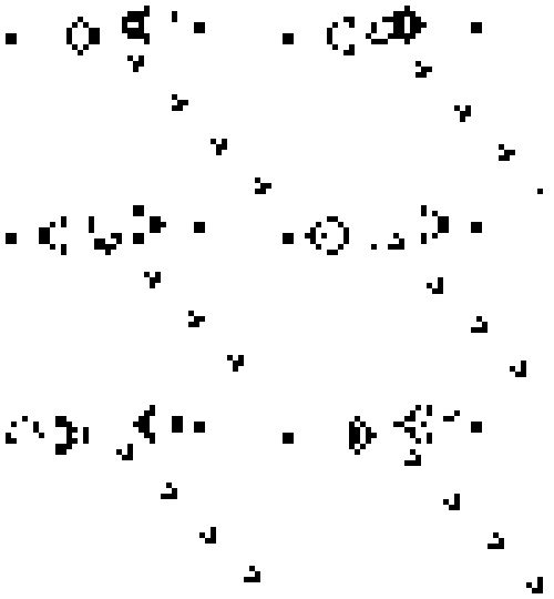
The Game of Life is a 2D CA due to John H. Conway. The CA can be seen as an abstract and qualitative description of how a population populate (or fail to populate) some environment. Cells have two possible states

• living (i.e., which means populated)
• dead (i.e., empty)

The rules are simple:

• an empty place is populated if it is surrounded by exactly 3 living cells
• a living cell die unless it is surrounded by 2 or 3 living cells (not to low for not being isolated, not to high for not suffocating)

The MGS implementation is straightforward: we use integers 0 and 1 to represent respectively dead and living cells to ease the count of living neighbor cells.

Let define the filename for JBView visualization

ofile := "/tmp/gol.jbv" ;;

Let define a initialization function populating a given grid g with 0 and 1 at random

fun populate_grid(g:Moore, size_x:int, size_y:int) = (
 
  for i = 0 to size_x do
    for j = 0 to size_y do
      g.(i * |E> + j * |N>) := random(2);
  g
 
) ;;

Let define the initial state S0

S0 := populate_grid(Moore:(),100,100) ;;

Let define the cellular automaton rules

trans rules = {
 
  // An empty cell is populated if it has exactly three alive neighbors
  0 as c / neighborsfold(add,0,c) == 3 => 1 ;
 
  // A living cell dies if it is not surrounded by two or three living cell
  1 as c / let nb_ngh = neighborsfold(add,0,c) in nb_ngh != 3 && nb_ngh != 2 => 0 ;
 
  // Implicit default rule: x => x
 
} ;;

Let define a function to save data for the viewer

fun output(S) = (
 
  ofile << " { " ;
  foreach c @ p in S do
    if c == 1
    then
      let (x,y) = sequify(p) in
        ofile << " { " << x << " " << y << " 0 0 0 } "
    fi;
  ofile << " }\n" ;
  S
 
) ;;

Let save data during the simulation

rules[iter = 200,
      prelude = output,
      interlude = output,
      postlude = output
     ](S0) ;;

The whole code follows

game_of_life.mgs

ofile := "/tmp/gol.jbv" ;;
 
fun populate_grid(g:Moore, size_x:int, size_y:int) = (
 
  for i = 0 to size_x do
    for j = 0 to size_y do
      g.(i * |E> + j * |N>) := random(2);
  g
 
) ;;
 
S0 := populate_grid(Moore:(),100,100) ;;
 
trans rules = {
 
  0 as c / neighborsfold(add,0,c) == 3 => 1 ;
 
  1 as c / let nb_ngh = neighborsfold(add,0,c) in nb_ngh != 3 && nb_ngh != 2 => 0 ;
 
} ;;
 
fun output(S) = (
 
  ofile << " { " ;
  foreach c @ p in S do
    if c == 1
    then
      let (x,y) = sequify(p) in
        ofile << " { " << x << " " << y << " 0 0 0 } "
    fi;
  ofile << " }\n" ;
  S
 
) ;;
 
rules[iter = 200,
      prelude = output,
      interlude = output,
      postlude = output
     ](S0) ;;

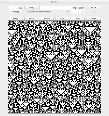
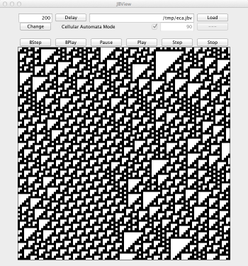
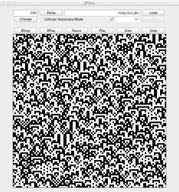
Elementary Cellular Automata (ECA) are 1D CA with two states and radius 1. There are exactly 256 possible specifications for the local rule. Each rule is identified by its Wolfram code which corresponds to a binary encoding of the rule. In the following code modify parameter number of transformation rules to consider some particular rule.

elementary_ca.mgs

ofile := "/tmp/eca.jbv" ;;
 
gbf grid = < d ; 100 d > ;;
 
S0 := map((fun x -> random(2)), iota(100, seq:())) following |d> ;;
 
fun nth_bit(num,n) = if n == 0 then num%2 else nth_bit(num/2,n-1) fi ;;
 
trans rules[number = 90] = {
 
  b => nth_bit(number, 4*neighbor(<d|,b) + 2*b + neighbor(|d>,b)) 
 
} ;;
 
fun output(S) = (
  for i = 0 to 100 do
    if S.(i * |d>) == 1 then
      ofile << " { " << i << " " << iteration << " 0 0 0 } "
    fi;
  S
) ;;
 
ofile << " { " ;;
rules[iter = 100,
      prelude = output,
      interlude = output,
      postlude = output
     ](S0) ;;
ofile << " }\n" ;;